In the previous post I introduced Reinforcement Learning and gave an overview of how it works in plain English. Next, let's look at how to write this definition as a mathematical problem.

Mathematically Formalising the Problem¶

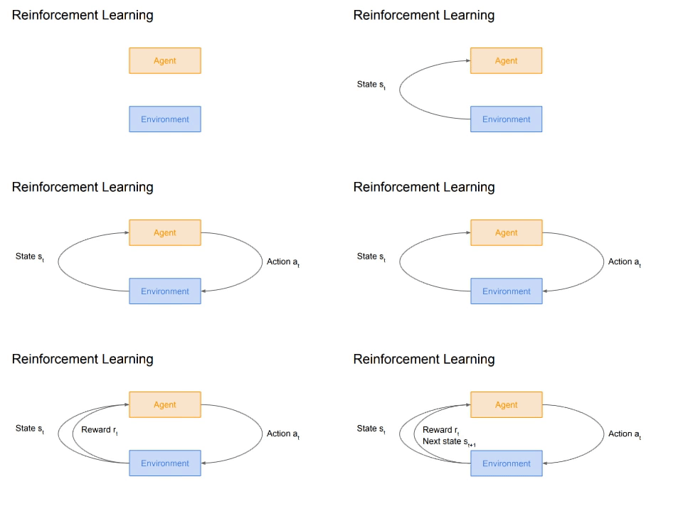
To solve the problem we need to define the problem! The animated loop shown below can be written using a mathematical formulation known as the Markov decision process (MDP).

The Reinforcement Learning Loop

An MDP satisfies the Markov property, which is that the current state completely characterizes the state of the world. Bear with me..

MDP Object Definitions¶

An MDP is defined by tuple of objects, consisting of:

$\mathcal{S}$, which is the set of possible states.
$\mathcal{A}$, our set of possible actions.
$\mathcal{R}$, our distribution of our reward, given a state-action pair. So it's a function mapping from state-action $\mapsto$ reward.
$\mathbb{P}$, which is a transition probability distribution over your next state, that you're going to transition to given your state-action pair.
$\gamma$, a discount factor, which is basically saying how much we value rewards coming up soon versus later on.

MDP Process¶

At time step $t=0$, the environment samples the initial state $s_0 \sim p(s_0)$
For $t=0$ until done (terminal state):
- Agent selects an action, $a_t$
- Environment samples a reward, $r_t \sim R( . | s_t, a_t)$
- Environment samples the next state, $s_{t+1} \sim P( . | s_t, a_t)$
- Agent receives the reward, $r_t$, and next state, $s_{t+1}$

🚨 New lingo: A policy, $\pi$, is a function that specifies what action to take in each state.

So our objective can be redefined as: Find the optimal policy, $\pi^*$, that maximises the cumulative (discounted) reward.

The term "discounted" is included here as we want to take into account our discount factor, $\gamma$, which balances how we value immediate vs. long term rewards.

This objective can be formulated as: $$\max\sum\limits_{t \ge 0} \gamma^t r_t$$

What about randomness?¶

How do we handle randomness? We have randomness in terms of the initial state that we're sampling, and in terms of this transistion probability distribution that will give us distributions over next states, and so on.

So we need to maximise the expected sum of rewards.

The optimal policy, $\pi^*$, is the policy which maximises this reward: $$\pi^* = \arg\max_{\pi}\mathbb{E}\left[\sum\limits_{t \ge 0} \gamma^t r_t|\pi\right]$$ with $$s_0 \sim p(s_0), a_t \sim \pi(\cdot|s_t), s_{t+1} \sim p(\cdot|s_t,a_t)$$

Note: $\mathbb{E}$ represents the expected value of a random variable

We can write our optimal policy $\pi^*$ as maximizing the expected sum of future rewards over policy's $\Pi$, where

initial state, $s_0$, is sampled from our state distribution
action, $a_t$, is sampled from our policy, given the state
next state, $s_{t+1}$, is sampled from our transition probability distributions